Authors: Faruk Gulban and Renzo Huber | Copyeditor: Lea Maria Ferguson | Published: May 2020
I have written about layered cakes and magnetic resonance imaging (MRI) before [here1, here2]. Following the *true millennial spirit* now it is time to broaden the menu by adding another delicious snack. And this time, this snack will taste even better because I have good company! A brilliant scientist (and a talented cook, too) @layer-fMRI and I are going to describe one of our recipes in this blog post (LN2_LAYERS program in LAYNII v1.5.5).
Fellow laminauts (lami-: layer, layering; -naut: traveler, voyager) are welcome to try this recipe and see the results for themselves.
Ingredients/Definitions
Following up on our previous blog post discussing the equi-volume principle, here we are going to lay-out one of the many ways of using this principle to generate cortical layers. But first, we need to clearly define the terms we are going to use:
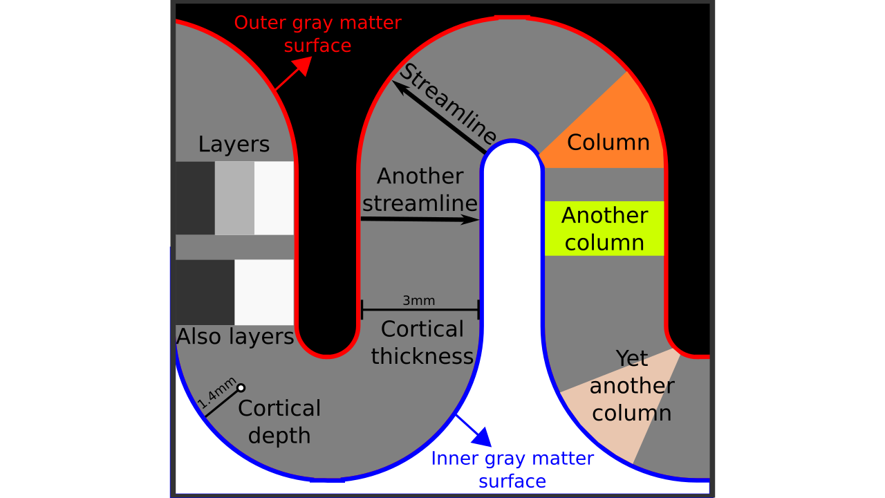
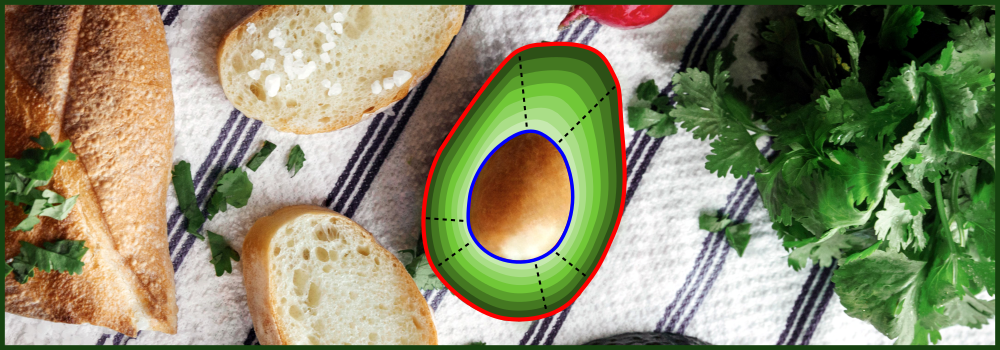
Figure 1. Terms visualized.
- Layer(s): According to the dictionary of etymology “a thickness of some material laid over a surface”. Everybody understands what “layers” mean intuitively, like wearing layers of clothes. However, some neuroscientists are sensitive about the “correct usage” of this term, referring strictly to neurobiological layers. Here we are *not* using layers to exclusively mean neurobiological layers, but instead to mean “a thickness of some voxels laid within cortical gray matter” which may or may not correspond to neurobiological layers. For more details on the “correct usage” of layers (or lack thereof) see this blog post.
- Inner gray matter surface: Portion of gray matter that mostly faces white matter.
- Outer gray matter surface: Portion of gray matter that mostly faces cerebrospinal fluid.
- Cortical thickness: Shortest distance in between outer and inner gray matter surfaces.
- Cortical depth: Distance from inner *or* outer gray matter surface, a portion of cortical thickness. Slightly different from “layer” because this term indicates a *quantitative measure* which may or may not be used to define the neurobiological layers.
- Streamline: A line that connects inner and outer gray matter surfaces based on some principle (not necessarily the shortest line).
- Column: A group of *voxels* that are successively penetrated by one or multiple streamlines. Not to be confused with neurobiological cortical columns which indicates a group of *neurons* not voxels.
- Unit column: Smallest unit of column that can be defined in a discrete lattice (ordered set of rectangular voxels) given the image resolution and topology of the cortex.
- Curvature: A measure of “how much a shape bends”. More specifically, here we are defining it as a measure of “how much a unit column bends”.
- Rim: A volume of cortical gray matter. Here, we specifically use this term to indicate our input image which consists of four integer values (0=irrelevant voxels, 1=outer gray matter surface voxels, 2=inner gray matter surface voxels, 3=pure gray matter voxels; see Figure 2 rightmost panel).
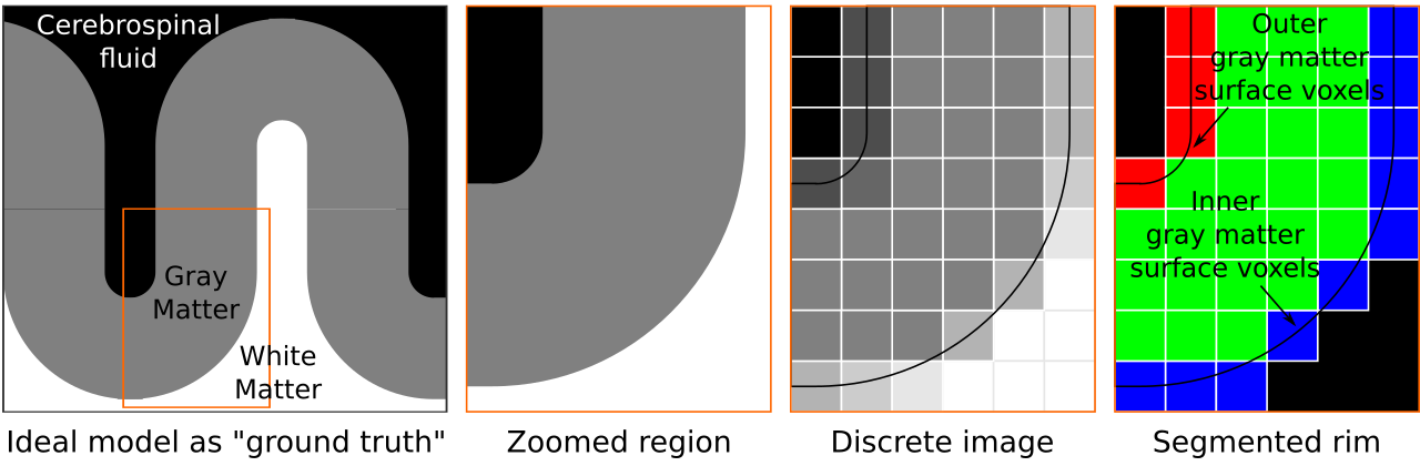
Figure 2. We start by conceptualizing an ideal toy brain model in the first pane. In this model boundaries are infinitesimally sharp and tissues are completely pure (i.e., no mixing of materials). Then we zoom in to a partially curved chunk of this toy model. Continuing, we sample this toy brain discretely on a cubic lattice. Each voxel color is determined by the exact partial voluming. This grayscale image is analogous to common MRI data. As the last step, given the discrete image, and knowing exactly where the tissue boundaries lie, we segment the cortical gray matter to generate our “rim” file. This rim file will frequently be referred while explaining our algorithm below.
Rules of the kitchen/Constraints
Every decision in image analysis comes with benefits and caveats. The following are the rules that we have followed when creating our algorithm (LN2_LAYERS):
- We are not allowed to upsample or interpolate the input image. This rule is employed because upsampling, interpolation etc. can always be added as a prior or separate step if one chooses to.
- We are not allowed to change the input data structure (i.e., no triangular or quad surface meshes). This rule is employed because each time the data structure is changed or augmented, we risk changing certain topographical qualities of our input image (this might be a topic for a future blog post).
- We are not allowed to do any fitting (aka no sphere fits to find curvature). This rule is employed in order to work without introducing dependencies of additional libraries that makes long-term software maintenance harder. And because an avocado toast can only be thoroughly enjoyed when its ingredients are obtained through sustainable sources.
- We are not allowed to use the Laplacian. This rule is employed in order to keep our mathematical operations as simple as possible (however, see Leprince et al. 2015 for an approach that uses the Laplacian).
- This algorithm has to work in 2D and 3D without extra operations or tweaks.
- This algorithm has to work with arbitrary brain topology. For instance, this algorithm should work with non-closed surfaces, thin slab data, and even with unconnected pieces of brain data with holes in them.
Step 1: Cortical depth
Aim: Find cortical depth of each gray matter voxel to outer gray matter surface and inner gray matter surface while preserving a basic set of topological qualities (e.g. not jumping across sulci).
Figure 3. Animation conveying the spatial intuition behind how we measure cortical depth. Closest outer (red) or inner (blue) gray matter surface voxels are found from each gray matter voxel (green).
Figure 4. Animation showing a more precise visualization of how cortical depth is computed.
Visualization in Figure 4 is done only for the outer (red) gray matter surface. Each voxel touching the initial surface is found through discrete jump steps following a precise access rule: looping through voxels from left to right then top to bottom while finding the neighbouring voxels clockwise starting from 12 o’clock. Such an accession rule gives a “handedness” to the connected voxels; therefore, there will be voxels connected to multiple surface voxels that are at equal distance, especially in curved areas. Here, we only allow each gray matter voxel to be connected to exactly one other voxel belonging to the given surface (inner or outer gray matter surface). Therefore, at the end, each gray matter voxel connects with exactly one outer and one inner gray matter surface voxel.
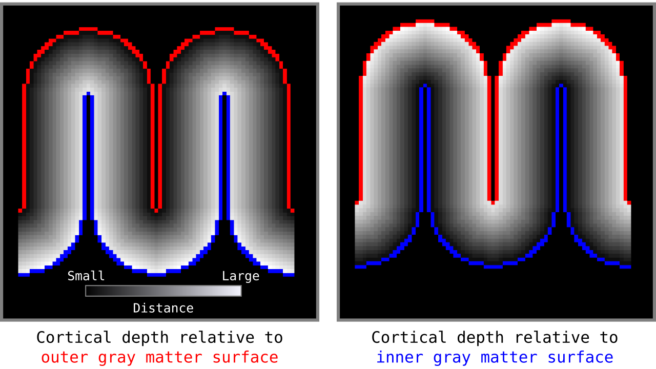
Figure 5. Example of the resulting cortical depths when applied to another higher resolution toy brain.
When we add the cortical depth relative to outer and inner gray matter surfaces, the resulting measurements are our cortical thickness values. There are many other ways to measure cortical thickness with different advantages and disadvantages. Here, for brevity, we are not discussing this further but inviting the curious reader to see Jones et al. (2000).
Step 2: Streamlines
Aim: Define exactly one streamline for every gray matter voxel.
Figure 6. Animation conveying the spatial intuition behind our streamline definition.
Figure 6 shows how one streamline per gray matter voxel (green) is defined by the closest outer (red) and the inner (blue) gray matter surface voxels. When there are multiple equally distant surface voxels, connection priority is given to the neighbouring voxel in “left-to-right then top-to-bottom” order.
Step 3: Columns
Aim: Define unit columns. A unit column *has to* touch at least one outer gray matter voxel and at least one inner gray matter voxel. A unit column might correspond exactly to one streamline where the cortex curvature is mostly straight (and thin). However, unit columns will often correspond to multiple streamlines when the cortex is curved (and thick).
Figure 7. Animation showing how the unit columns are defined. Note that each outer gray matter surface voxel (red) is (being) accessed to check the streamlines originating here (black lines) and reaching to the inner gray matter surface voxels (blue). Each gray matter voxel (indicated by circles) that a given set of streamlines has passed through is used to define a unit column. The number within the red voxels denote how many blue voxels the columns have reached. These numbers are also computed from the blue voxels to the red voxels and used to determine local curvature type (sulcus or gyrus). However, these numbers are not relevant for the rest of the algorithm.
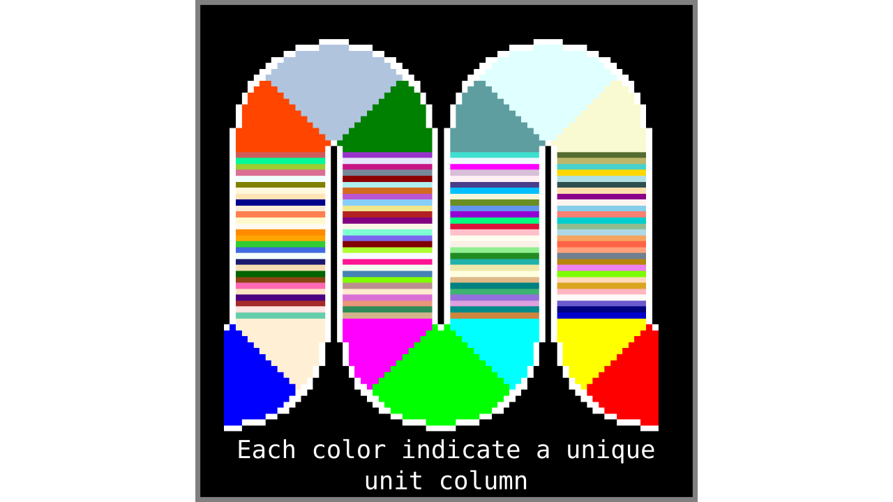
Figure 8. Showing what computing unit columns produce when applied to another higher resolution toy brain.
Our unit column definition is immediately useful in the following ways:
- The unit columns do not overlap and they exhaustively cover all gray matter voxels. Note that the unit columns will cover larger volumes in curved regions (sulci and gyri).
- It is straightforward to calculate the number of unit columns. The number of unit columns is equal to the number of inner gray matter surface voxels when on a gyrus plus the number of outer gray matter surface voxels when on sulcus (completely straight pieces of cortex can either be counted as gyrus or sulcus without changing the result).
- It is well defined given the discrete geometry of the input image.
- [Bonus] It is extremely fast to compute by using pointers (the extra fair-trade sesame on top).
Step 4: Normalize cortical depth
Divide measured cortical depths with cortical thickness for each gray matter voxel. This step results in *normalized cortical depths* with values only being in between 0-1 range. We compute the normalized cortical depths relative to the inner gray matter surface, therefore values close to 0 indicate deep layers and 1 indicate superficial layers. The general aim of this step is to be able to exploit some useful properties of this metric space. For instance having a guarantee on measurements being in between 0-1 range is more useful compared to 0-infinity range because we can easily quantize this space to generate desired number of output layers For instance realize that normalized cortical depth of 0.5 always indicates middle gray matter surface.
Step 5: Generate equi-distant layers
Our main destination is to reach equi-volume layering; however, we can take a quick detour to generate our beloved equi-distant layers as a bonus. It’s like toast without the avocado. If you are really hungry (or out of ripe avocados), it is also a joyful snack.

Figure 9. Animation showing equi-distant layers after quantizing (assigning a range of values to an integer) normalized cortical depths.
Note that the number of layers can be determined arbitrarily. However, given the image resolution, some layers might not show up in the end. For instance, if you have a straight piece of cortex with 3 voxels but want to have 10 equi-distant layers, it is not possible to have all 10 layers represented within those 3 voxels. To do this, you need to first resample your input image to a higher resolution (using your favorite interpolation method). We leave determining the right amount of layers to the user. Try `LN2_LAYERS -rim rim_M.nii -nr_layers 3` command to test it for yourself and play with different numbers of layers.
Step 6: Magic numbers (Chef’s special sauce)
Warning!: This special sauce was concocted upon visiting the library of Miskatonic University. We strongly advise the faint-hearted readers to not read this step alone at night.
Aim: Manipulate the available metric space (normalized cortical depths from Step 4) in such a way that when quantized (like in Step 5) it automagically yields equi-volume layers.
We first count the number of voxels that fall below 0.5 normalized cortical thickness and separately count the voxels that fall above it for each unit column. In the next step, we imagine the counted voxels as weights to be placed on a two-armed weighing scale. Then, we ask the question: “how much, and to which direction, do we need to shift the center of the scale so it’s perfectly balanced?”.
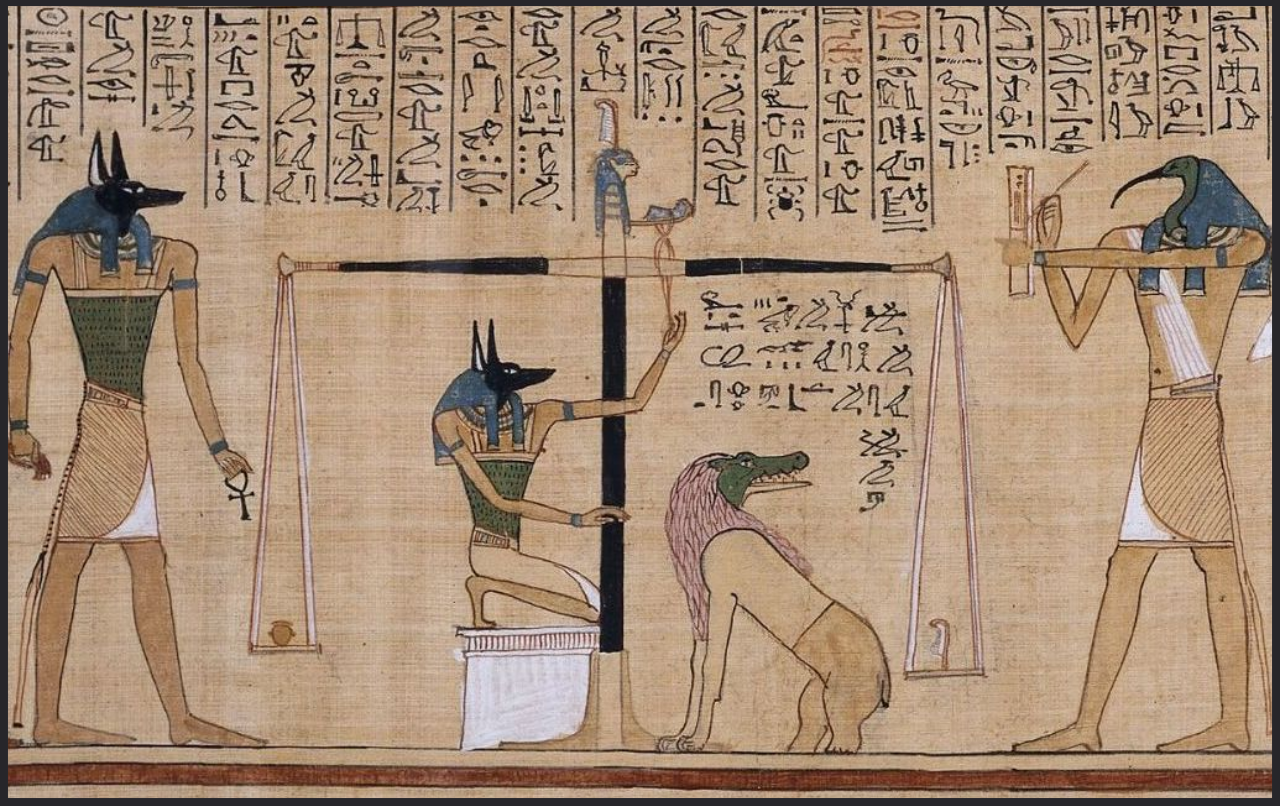
Figure 10. “The jackal-faced god Anubis supervising the weighing of a dead man’s heart, while the ibis-headed messenger-god Thoth on the right records the result.” (Gombrich, 1950). The two-armed weighing scale measures the scribe’s heart against the feather of truth (Book of the Dead, circa 1285 BC). Using a similar technique, here we are measuring the weight of voxels below the middle gray matter surface against the weight of voxels above.
The answer to this question is our magic number. Let’s call these magic numbers “equi-volume factors”. Different unit columns will have different equi-volume factors depending on the local curvature (although we did not even compute the curvature!). These equi-volume factors (denoted by Ω, a value within 0-1 range) are very useful when plugged into the following equation:
d1_new = (d1*Ω) / (d1*Ω + d2*(1-Ω))
where d1 is the normalized cortical depth relative to the inner gray matter surface, and d2 is the normalized cortical depth relative to the outer gray matter surface voxel within each gray matter voxel. d1_new is our new metric that, when quantized, generates equi-volume layers. For the purist reader, if we had infinite resolution and wanted to have an infinite number of equi-volume layers, this metric would still give us equi-volume layers (within each unit column). However, an infinite number of equi-volume layers is an oxymoron because the concept of volume does not exist when the layers are infinitesimally thin.
Note: The intuition behind this section comes from a lesser known piece of geometry involving multidimensional triangles. For brevity, we are sparing further details but opt for giving two hints to the curious reader: Möbius (1827), Gulban (2018).
Step 7: Generate equi-volume layers
After transforming our normalized cortical depth metric into a equi-volume yielding metric in the previous step, we can quantize this metric to generate our initial equi-volume layers.
Figure 11. Animation showing the *intermediate* equi-volume layering results. At this stage, smooth transitions between unit columns are not yet enforced (see the next step).
As you can see, there is a small problem. Transitions between curved and straight regions of the cortex are very sharp. While these layers fulfill the equi-volume principle, this does not seem to be biologically plausible. Therefore, we still need to enforce some amount of smoothness before generating the final equi-volume layers.
Step 8: Transition smoothing
Aim: Make the discontinuous transitions near the unit column edges continuous.
Figure 12. Animation showing the iterative process we use to smooth out the harsh transitions between unit-column edges. This iterative smoothing is inspired by the process of general heat diffusion.
You can see that the layer transitions between curved and straight regions become smoother over time. We use the smallest possible smoothing kernel defined at the input image resolution to avoid leakage across sulci and gyri. For the observant reader, we are not directly smoothing the quantized layers but smoothing within Step 7. Precisely, we are smoothing the equi-voluming factors to diffuse the nonlinear metric space transformations over spatial space.
Currently, the biologically plausible amount of smoothness between geometrically well-defined columns is unknown. Therefore, we leave determining the “right amount of smoothness” to the user (see usage of `-iter_smooth` flag in LN2_LAYERS program). Note that excessive amounts of smoothing (e.g. 10000 iterations) will take longer due to the iterative nature of our smoothing method. We have chosen 100 smoothing iterations as our default, which seems to yield good enough results in most of our tests. We did not yet stumble upon a use case where this step takes a prohibitively long time. Note that the number of smoothing iterations is quadratically coupled to the spatial extent of this iterative smoothing, i.e. 64 iterations result in a FWHM that is twice as big as 8 iterations.
Step 9: Et voilà!
Figure 13. Animation showing the input (left) and the resulting main outputs. You can produce all the above mentioned output images by running `LN2_LAYERS -rim rim_M.nii -nr_layers 3 -equivol -iter_smooth 100` command on your own computer (rim_M.nii is available inside LAYNII test_data folder). Note that the equi-distant metric and equi-volume metric outputs give you access to see exactly what is being quantized.
Outro
Using our algorithm on an empirical MR image, we get the following result:
Figure 14. Animation showing the difference between equi-distant and equi-volume layering outputs at 0.2 mm isotropic resolution. Note that in this example the algorithm operates on a 3D image with no additional changes. More precisely, we used `LN2_LAYERS -rim Ding_V1_rim.nii.gz -nr_layers 3 -equivol -iter_smooth 100` command as implemented in LAYNII v1.5.5 to produce both layerings.
To test an extreme case, we ran our algorithm on a 0.1mm isotropic whole brain image (BigBrain, histology image):
Figure 15. Animation showing layering differences in an extreme case (considering practicable MRI image resolutions and coverage). Here we used the BigBrain dataset (Amunts et al. 2013) at 0.1 mm isotropic resolution. We thank Konrad Wagstyl for providing the segmentation from Wagstyl et al. (2020). See ‘Algorithm Overview’ section for performance tests (e.g. 0.2 mm iso. whole brain takes around 12 minutes to produce equi-volume layers).
Evidently the algorithm works (tasty!). However, some important questions remain:
- How well does it work? (How filling is it?)
- Under which circumstances does it fail? (Indigestion?)
- Are there any alternative equi-volume layering methods implemented in LAYNII? (Blue cheese toast?)
We are going to answer all these questions in due time. But for now, if you can excuse us, we will enjoy our avocado toasts (possibly with some specialty coffee on the side)… In the meanwhile, stay tuned for more recipes!
Algorithm overview
Understanding an algorithm/recipe gradually develops at different levels of detail. Similar to seeing an island on the horizon and slowly recognizing more details as you sail closer, the transition from being a user to a developer requires recognizing the tiniest of details (upon lots of rowing). In order to further help fellow layer-enthusiasts, in this section, we offer *a bird’s eye view* of our algorithm that conveys an intermediate level of detail in between our source code and the rest of this blog post.
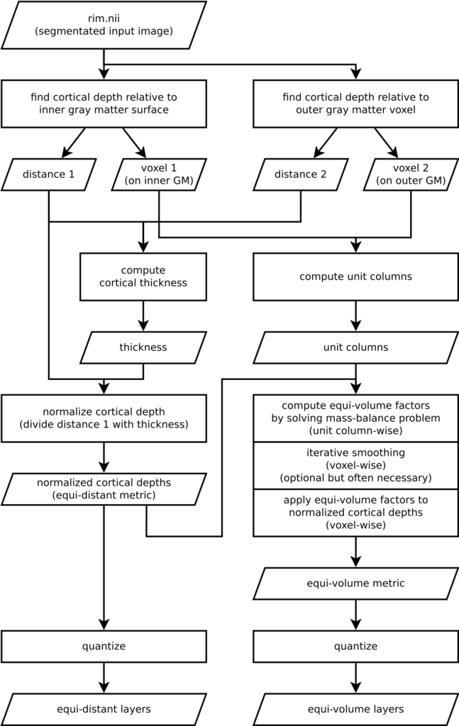
Figure 16. Flowchart of LN2_LAYERS as implemented in LAYNII v1.5.5.
Performance tests
| Whole brain res. | RAM usage | Equi-distant layers | Equi-volume layers |
|---|---|---|---|
| 0.50 mm iso. | ~1.5 GB | ~8 sec. | ~46 sec. |
| 0.45 mm iso. | ~2 GB | ~10 sec. | ~1 min. |
| 0.40 mm iso. | ~3 GB | ~15 sec. | ~1 min. 30 sec. |
| 0.35 mm iso. | ~4 GB | ~22 sec. | ~2 min. 15 sec. |
| 0.30 mm iso. | ~7 GB | ~35 sec. | ~3 min. 30 sec. |
| 0.25 mm iso. | ~11 GB | ~1 min. | ~6 min. 15 sec. |
| 0.20 mm iso. | ~22 GB | ~2 min | ~12 min. 15 sec. |
A quick test of system requirements using `LN2_LAYERS -rim input.nii.gz -equivol -iter_smooth 100` command (as implemented in LAYNII v1.5.5). Numbers would change depending on the specific hardware. For instance if you do not have enough RAM, it would take significantly longer or run out of memory (physical and virtual ) and terminate before completion. For now we are not doing any parallel processing or memory usage optimization. Therefore, there is room for significant performance improvements in the future. We might invest time on this depending on user feedback but it is a not high priority.
How to contribute?
If you have any issues when using LAYNII, or want to request a new feature, we are happy to see them posted on our github issues page. Please employ this as your preferred method (instead of sending individual emails to the authors), since fellow researchers might have similar issues and suggestions.
References & inspirations
- Crane, K. (2020). Discrete Differential Geometry – Lecture 15: Curvature of Surfaces [video lecture].
- Stam, J. (2015). The art of fluid animation. [book]
- Waehnert, M. D., Dinse, J., Weiss, M., Streicher, M. N., Waehnert, P., Geyer, S., Turner, R., Bazin, P.-L. (2014). Anatomically motivated modeling of cortical laminae. NeuroImage, 93 Pt 2, 210–220. [Link]
- Kemper, V. G., De Martino, F., Emmerling, T. C., Yacoub, E., & Goebel, R. (2018). NeuroImage, 164, 48–58. [Link, see Figure 1]
- Polimeni, J. R., Renvall, V., Zaretskaya, N., & Fischl, B. (2018). Analysis strategies for high-resolution UHF-fMRI data. NeuroImage, 168(April), 296–320. [Link, see “Predicting geometry of columns and layers” section]
- Leprince, Y., Poupon, F., Delzescaux, T., Hasboun, D., Poupon, C., & Riviere, D. (2015). Combined Laplacian-equivolumic model for studying cortical lamination with ultra high field MRI (7 T). 2015 IEEE 12th ISBI, 2015-July, 580–583. [Link]
- Jones, S. E., Buchbinder, B. R., & Aharon, I. (2000). Three-dimensional mapping of cortical thickness using Laplace’s equation. Human Brain Mapping, 11(1), 12–32. [Link]
- Möbius, A. F. (1827). The barycentric calculus. [from book “Möbius and his band” by Fauvel, Flood, and Wilson; a source of intuition for Step 6 for that one in a million person who wants to dig deeper]
- Gulban, O. F. (2018). The relation between color spaces and compositional data analysis demonstrated with magnetic resonance image processing applications. Austrian Journal of Statistics, 47(5), 34–46. [Link, another source of intuition for Step 6]
- Ding, S. L., Royall, J. J., Sunkin, S. M., Ng, L., Facer, B. A. C., Lesnar, P., … Lein, E. S. (2016). Comprehensive cellular-resolution atlas of the adult human brain. Journal of Comparative Neurology. [Link]
- Amunts, K., Lepage, C., Borgeat, L., Mohlberg, H., Dickscheid, T., Rousseau, M.-E., Bludau, S., Bazin, P.-L., Lewis, L. B., Oros-Peusquens, A.-M., Shah, N. J., Lippert, T., Zilles, K., & Evans, A. C. (2013). BigBrain: an ultrahigh-resolution 3D human brain model. Science (New York, N.Y.), 340(6139), 1472–1475. [Link]
- Wagstyl, K., Larocque, S., Cucurull, G., Lepage, C., Cohen, J. P., Bludau, S., Palomero-Gallagher, N., Lewis, L. B., Funck, T., Spitzer, H., Dickscheid, T., Fletcher, P. C., Romero, A., Zilles, K., Amunts, K., Bengio, Y., & Evans, A. C. (2020). BigBrain 3D atlas of cortical layers: Cortical and laminar thickness gradients diverge in sensory and motor cortices. PLOS Biology, 18(4), e3000678. [Link]
- Huber, L., Gulban, O.F. (2020). LAYNII v1.5.5. Zenodo. [Link]
Thanks
We thank Rainer Goebel for his encouragement on this endeavor and discussions on various layering algorithms over 2013-2019 period. We thank Konrad Wagstyl for providing the BigBrain segmentation and our discussion on the column shapes. We thank Ilkay Isik and Mario Eduardo Archila-Melendez for their comments and suggestions with regards to language and visuals.
Visuals
Images and animations that are not referenced above are created by the authors and licensed under CC BY 4.0 license.