Authors: Faruk Gulban | Copyeditor: Lea Maria Ferguson | Published: May 2019
In the second part of my blog posts about cake-inspired layer-MRI, I am going to inspect some tasty ring-shaped layered cakes.

Three rings to rule them all
This time I would like to expand upon for the second claim [II] about partial voluming that was mentioned in my previous post:
… The primary visual cortex is approximately three voxels thick. The average profiles … however are very smooth and hence appear to be highly interpolated versions of (effectively) three-point data… This smoothness is caused by a partial volume effect when averaging all profiles together. The voxel grid is arbitrarily oriented with respect to … cortex (i.e. [I] a voxel boundary may or may not be aligned with a tissue boundary, [II] voxel and tissue boundaries may intersect at an arbitrary angle, etc.). Therefore … all voxels together will uniformly sample the cortical depth (as opposed to only sampling the cortex at three depths).
Koopmans, Barth, Orzada, Norris (2011)
I have developed the following method to approach the problem of on partial voluming due to the angled tissue boundary-voxel intersection highlighted above:
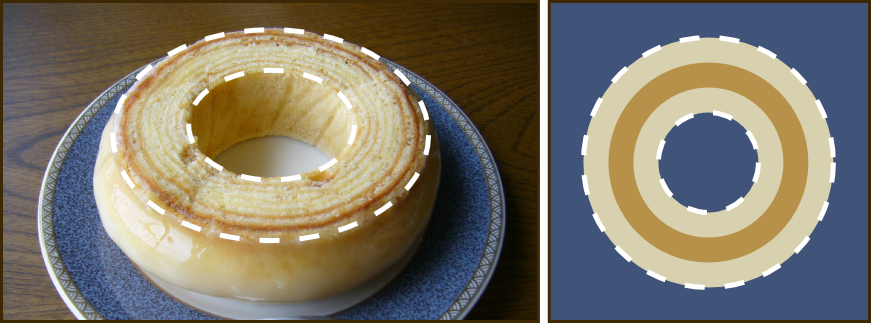
- Create an ideal curved cake (a ring brain) with a few high contrast layers (for simplicity I have chosen 3 here).
- Position sampling grid in a way that one voxel aligns with each layer almost perfectly along the cardinal axes (left-right, down-up).
- Move the sampling grid a tiny bit each time to see how the ideal object looks across different alignments of voxel boundary and tissue boundary.
- Select best and worst cases by looking at the amount of blurring across the ring brain.
Figure 2.
- Position a line that will be used to sample layer profiles. Let’s call this sampling line.
- Move the sampling line one degree at a time along the ring-brain to sample varying voxel-tissue boundary intersections.
The layer profiles along the cardinal axes (left-right, down-up) approach the ideal profile in the best case sampling. As the angle between the sampling line the cardinal axes diverge, the layer profiles become quite distorted (see the video in the right column). Additionally, the worst case sampling shows that even though the angle between the sampling line and the cardinal axes is small we cannot see the ideal layer profile when the grid is misaligned to layers boundaries. Having observed these distortions, on the other hand, you can also appreciate that there are moments where the layer profiles resemble the ideal case more closely.
It seems that our chances of seeing the ideal layering decreases with partial voluming due to grid alignment and angled tissue boundary-voxel intersection even in these simple cake-inspired models. While this is, of course, not surprising, I think that seeing the extent of these effects clearly on toy models is useful to develop a spatial understanding. For instance, now I am bit more careful of interpreting one layer profile type changing into another as opposed to seeing the transition between two different areas with different layer profiles. This is because I know that this observation might just be due to partial voluming.
Local vs. global profiles
I would like to emphasize that in these two posts I was mostly looking at local layer profiles instead of the average layer profiles in an area. In the next post I would like to focus on differences between local layer profiles and global layer profiles (somewhat similar to Figure 4 of Polimeni, Renvall, Zaretskaya, Fischl, 2017) and how these profiles can be used to distinguish different brain areas.
References/Inspirations
- Koopmans, P. J., Barth, M., Orzada, S., & Norris, D. G. (2011). Multi-echo fMRI of the cortical laminae in humans at 7T. NeuroImage, 56(3), 1276–1285. [Effective resolution section, Figure 2 and 3]
- Polimeni, J. R., Renvall, V., Zaretskaya, N., & Fischl, B. (2017). Analysis strategies for high-resolution UHF-fMRI data. NeuroImage, (April), 1–25. [Figure 4 and 5]
While I was writing this, I have stumbled upon a similar toy model in a recent paper. It is used in a different way and for a different purpose, but I like it nonetheless:
- van Mourik, T., van der Eerden, J. P. J. M., Bazin, P.-L., & Norris, D. G. (2019). Laminar signal extraction over extended cortical areas by means of a spatial GLM. PLOS ONE, 14(3), e0212493. [Figure 3]
Thanks
I would like to thank to layer-fMRI and model-fMRI for the lively discussions that propelled me to generate the animations and write this up.
Visuals
Images and animations that are not referenced above are created by the author and licensed under CC BY 4.0 license.