
Authors: Faruk Gulban and Renzo Huber | Copyeditor: Lea Maria Ferguson | Published: October 2020
If you ask yourself the following question, this post is a must-read for you: “I have ultra/mega/super/high resolution 2D or 3D brain images and I want to analyze cortical columns. Where do I start from?”
Neuroscience people do stuff with cortical columns. They also do stuff with cortical layers whenever they do stuff with the cortical columns. Renzo and I have already described the first half of this process, namely an algorithm (LN2_LAYERS) to generate cortical layers here. Therefore, now is the time to describe the other half: an algorithm to generate an arbitrary number of cortical columns (LN2_COLUMNS). Possibly the simplest algorithm out there!
Kitchen rules
- Stay in the voxel space. All operations have to be done in the volume space using good old rectangular voxels (no surfaces, no triangular meshes).
- Work on 2D and 3D images. Column generation must work in 2D and 3D images by using the same principles. No additional tweaks, parameters, or massaging are allowed.
Ingredients
Now that we have laid down the kitchen rules, it is time to list our ingredients:
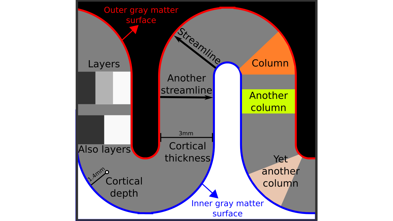
- Segmented rim file: A volume of cortical gray matter. Here, we specifically use this term to indicate our input image which consists of four integer values (0=irrelevant voxels, 1=outer gray matter surface voxels, 2=inner gray matter surface voxels, 3=pure gray matter voxels; see previous post Figure 1).
- Middle gray matter voxels: A subset of gray matter voxels that lies on a surface at equal distance from the inner and outer gray matter borders. We are going to generate this file by using LN2_LAYERS on the segmented rim file. You can go back to the previous blog post (here) to understand how this image is computed.

Illustration of the original meaning of columns.
- Column(s): According to the dictionary of etymology “a pillar, long, cylindrical architectural support”. Everybody understands what “columns” mean intuitively. Columns are long and thin things. However, some neuroscientists are sensitive about the “correct usage” of this term, referring strictly to neurobiological columns, minicolumns, hypercolumns etc… Here we are *not* using columns to exclusively mean neurobiological columns, but instead to mean “a set of voxels that look long and thin” which may or may not correspond to neurobiological columns.
- Desired number of columns: Some want more, some want fewer, others want both simultaneously. You might determine this number based on your visual intuition. Ideally columns are taller than they are wide. Therefore, as a rule of thumb: Ensure that the generated columns look taller than they are wide on average. ‘Taller than they are wide’ means that the average number of voxels that lie perpendicular to the cortical surface is greater than the average number of voxels that lie parallel to the cortical surface. In our algorithm, there are no guarantees that the generated columns will obey this rule (for now). However, this number is not hard to determine upon running the algorithm and visually inspecting the results. One can also deduce the desired number of columns by considering a few neurobiological measurements. For instance, the human cerebral cortex has a surface area of about ~2400 cm2 on average (Toro et al. 2006, Figure 1). Thus, the surface area of one hemisphere comes about ~1200 cm2. If one wants average column diameters to be around 0.8 mm wide, then you can consider the following relation:
nr_columns = surface_area / column_surface_area. Note that cylindrical columns with 0.8 mm diameter (0.4 mm radius) would have a surface area ~0.5 mm2 (coming from the circle area formulaarea = π ⋅ r2). Thereforenr_columns = 120000 mm2 / 0.5 mm2givesnr_columns = 240000. When conducting whole brain MRI experiments on living humans, we are far away from accurately and precisely measuring from neurobiologically plausible columns due to the image resolution constraints. Therefore, practically you might want to create fatter columns as an approximation. For example ~2 mm in diameter columns would give around 38000 columns for one hemisphere. These columns would still mostly be “taller than they are wide” based on the assumption that the human cortex is 2.5 mm thick on average.
Bake it till you make it
We have prepared the ingredients, now we start working with them:
- Take one of the middle gray matter voxels and register it to a list of “cortical column centroids”.
- Measure the distance of every other voxel (or of all respective voxels) to the voxels within the “cortical column centroids” list. In case of multiple distance measurements, the shortest distance (always) wins.
Figure 1: Animated snapshots of computed middle gray matter geodesic distances from Step 2 after each iteration.
- Add the farthest-away voxel to the “cortical column centroids” list.

Figure 2: Animated snapshots of newly determined column centroids from Step 3 after each iteration.
- Go back to step 1 and iterate until the “cortical column centroids” list has the desired number of cortical columns.
- Grow Voronoi cells from the “cortical column centroids” list.
Figure 3: Voronoi cells grown from the middle gray matter column centroids found in Steps 1 to 4.
We call this algorithm iterative farthest point Voronoi subdivisions:
- Iterative because it generates the desired number of columns one after another,
- Farthest point because the location of the next column centroid is determined by its topographical distance from the other column centroids,
- Voronoi subdivisions because the generated column centroids (singular voxels) are turned into columns (clusters of voxels) through subdividing the input topology (segmented rim file) by Voronoi diagramming.
Simple sweetness
It is possible to scale up this simple recipe to (yet) another dimension! And the good news is that it still tastes as sweet as when prepared in 2D!
Figure 4: Results of LN2_COLUMNS in a 3D partial coverage image (from Ding et al. 2016). More precisely, e.g. we used LN2_COLUMNS -rim Ding_V1_rim.nii.gz -midgm Ding_V1_rim_equidist_midgm.nii.gz -nr_columns 1000 to generate 1000 columns.
Figure 5: Results of LN2_COLUMNS on a whole brain image 0.1 × 0.1 × 0.1 mm resolution ( data from BigBrain, Amunts et al. 2013). We thank Konrad Wagstyl for providing the segmentation from Wagstyl et al. (2020).
LN2_COLUMNS is truly the choice of high resolution neuroimaging connoisseurs… 🍴👌
Serving suggestions

LN2_COLUMNSis a new and different program. Do not confuse it with what is used in Renzo’s older blog post (https://layerfmri.com/columns/).- When does
LN2_COLUMNSnot work properly? When the desired number of columns is too many so that the columns do not span the whole cortical depth in curved regions. - I have too few columns, can I increase the number of columns without processing all from start? Yes you can. Use
LN2_COLUMNSwith-centroidsargument in the command line. See the help menu for further details (LN2_COLUMNS -help) - I have too many columns, can I reduce the number of columns without processing all from start? Yes you can. Use
LN2_COLUMNSwith-centroidsargument in the command line. See the help menu for further details (LN2_COLUMNS -help). LN2_COLUMNSdoes not find the *right* column locations, can I initialize it with columns centroids that I draw myself manually? Yes you can. UseLN2_COLUMNSwith-centroidsargument in the command line.LN2_COLUMNSlabels columns centroids iteratively starting from 1. Therefore, for example, you can prepare a centroids file with column centroids positions labeled manualy from 1 to 10 and then let it find the rest of the columns.- A common mistake is to look at 2D slices of a 3D image to understand whether the column shapes make sense. Do not do this. Columns of 3D brain images live in 3D space. Escape from Plato’s cave to comprehend the 3D column shapes turthfully by e.g. using ITK-SNAP’s quick 3D rendering tool (after loading
LN2_COLUMNSoutput as a segmentation file).
Algorithm overview
Understanding an algorithm/recipe gradually develops at different levels of detail. Similar to seeing an island on the horizon and slowly recognizing more details as you sail closer, the transition from being a user to a developer requires recognizing the tiniest of details (upon lots of rowing). In order to further help fellow layer-enthusiasts, in this section, we offer *a bird’s eye view* of our algorithm that conveys an intermediate level of detail in between our source code and the rest of this blog post.
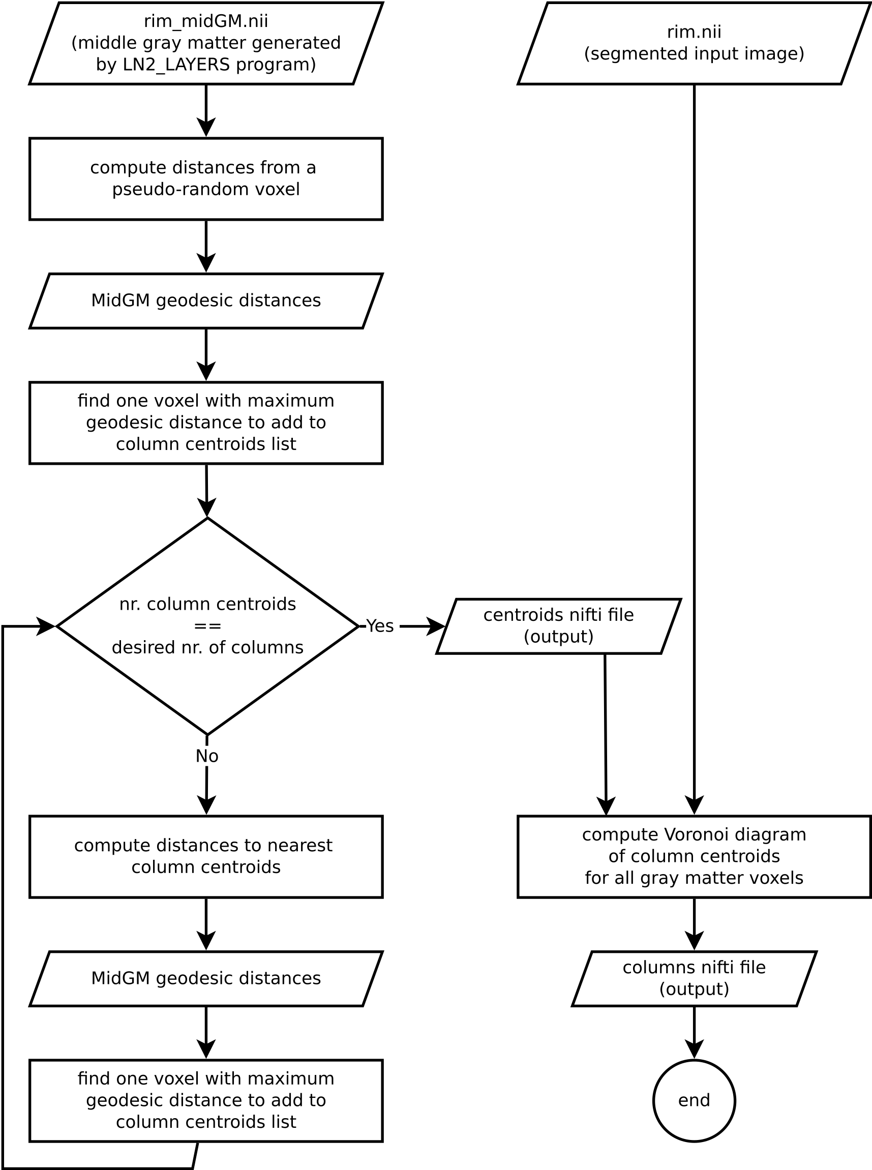
Figure 6. Flowchart of LN2_COLUMNS as implemented in LAYNII v1.6.0.
Performance tests
| Whole brain res. | RAM usage | Number of generated columns | Duration |
|---|---|---|---|
| 0.20 mm iso. | <8 GB | 100 | ~15 min. |
| 0.20 mm iso. | <8 GB | 1000 | ~81 min |
| 0.20 mm iso. | <8 GB | 10000 | ~540 min |
| 0.50 mm iso. | <8 GB | 1000 | ~12 min. |
| 0.50 mm iso. | <8 GB | 40000 | ~360 min |
How to contribute?
If you have any issues when using LAYNII, or want to request a new feature, we are happy to see them posted on our github issues page. Please employ this as your preferred method (instead of sending individual emails to the authors), since fellow researchers might have similar issues and suggestions.
References & inspirations
- Toro, R., Perron, M., Pike, B., Richer, L., Veillette, S., Pausova, Z., & Paus, T. (2008). Brain size and folding of the human cerebral cortex. Cerebral Cortex, 18(10), 2352–2357. [Link]
- Ding, S. L., Royall, J. J., Sunkin, S. M., Ng, L., Facer, B. A. C., Lesnar, P., … Lein, E. S. (2016). Comprehensive cellular-resolution atlas of the adult human brain. Journal of Comparative Neurology. [Link]
- Amunts, K., Lepage, C., Borgeat, L., Mohlberg, H., Dickscheid, T., Rousseau, M.-E., Bludau, S., Bazin, P.-L., Lewis, L. B., Oros-Peusquens, A.-M., Shah, N. J., Lippert, T., Zilles, K., & Evans, A. C. (2013). BigBrain: an ultrahigh-resolution 3D human brain model. Science (New York, N.Y.), 340(6139), 1472–1475. [Link]
- Wagstyl, K., Larocque, S., Cucurull, G., Lepage, C., Cohen, J. P., Bludau, S., Palomero-Gallagher, N., Lewis, L. B., Funck, T., Spitzer, H., Dickscheid, T., Fletcher, P. C., Romero, A., Zilles, K., Amunts, K., Bengio, Y., & Evans, A. C. (2020). BigBrain 3D atlas of cortical layers: Cortical and laminar thickness gradients diverge in sensory and motor cortices. PLOS Biology, 18(4), e3000678. [Link]
- Huber, L., Gulban, O.F. (2020). LAYNII v1.6.0. Zenodo. [Link]
Thanks
We thank Rainer Goebel for his encouragement on this endeavor and discussions on various column generation algorithms over 2013-2019 period. We thank Konrad Wagstyl for providing the BigBrain segmentation and our discussion on column shapes.
Visuals
,_May_2010.jpg)
.jpg)
Images and animations that are not referenced above are created by the authors and licensed under CC BY 4.0 license.