Authors: Faruk Gulban and Renzo Huber | Copyeditor: Lea Maria Ferguson | Published: June 2021
Flat things are simple. Cortical things (layers) are convoluted which makes them complicated. Then, how can we turn cortical things into flat things? If you are struggling with flattening your convoluted cortex chunks this post is for you! We are going to explain how to make (and bake!) flat chunks of brain using two new additions to LayNii (v2.1.0): LN2_MULTILATERATE and LN2_PATCH_FLATTEN.
Figure 1: Do you want to learn how to flatten 3D brain chunks to see their layers? Follow along this blog post to see a step by step description of how to do so.
Why should I care?
There are at least 3 reasons for you to continue reading if you are a high-resolution neuroimaging researcher (doing layer-fMRI, histology etc.):
- Nifti goes in, nifti comes out! Our program does not need anything other than simple nifti files as inputs. All inputs and outputs are in the common nifti format.
- Plays well with partial coverage (a.k.a. brain chunks)! Our algorithm is tailored to operate on cortical chunks. You do not need to acquire or segment whole brain images.
- Easy to integrate into your working pipeline! Are you using Freesurfer, BrainVoyager, Nighres, AFNI etc. already? Our programs can be integrated into your pipelines easily and they will play along well with the other software.
Ingredients
This section describes the user inputs to LN2_MULTILATERATE algorithm.
- MRI Data: A 3D nifti image of some contrast (T1-w, T2*-w, histology etc). Here we are going to use a chunk of human V1 image from Ding et al. (2016). This image is at 0.2 mm isotropic resolution and has great T2*-w contrast to reveal some of the cortical gray matter layers.
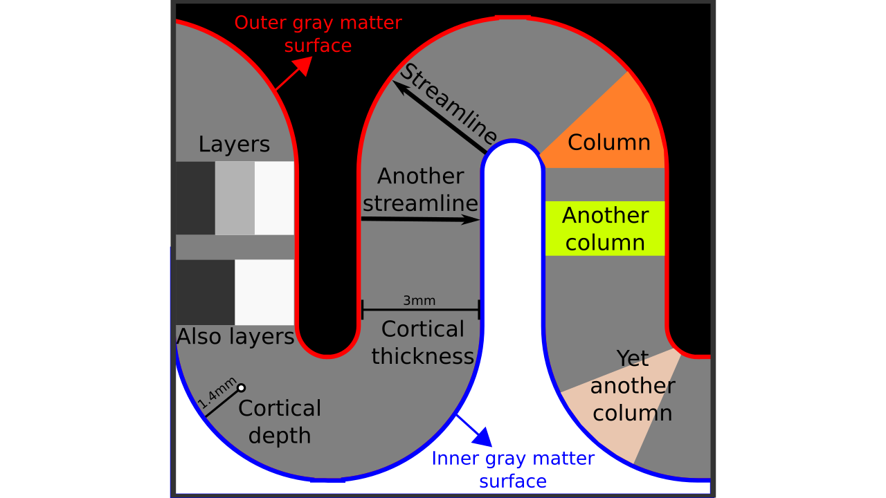
- Segmented rim file: A volume of cortical gray matter. Here, we specifically use this term to indicate our input image which consists of four integer values (0=irrelevant voxels, 1=outer gray matter surface voxels, 2=inner gray matter surface voxels, 3=pure gray matter voxels; see previous post Figure 1). If you already have segmented images from other software (e.g. Freesurfer, BrainVoyager, FSL, AFNI, Nighres); you can easily convert your segmented images into LayNii’s “rim file” specification by using our LN2_RIMIFY program.
- Control points: This is a modified middle gray matter file. Here we computed our middle gray matter voxels using `LN2_LAYERS -rim Ding_data.nii.gz` command from LayNii. The middle gray matter voxels (denoted with “*midgm” suffix in output of LN2_LAYERS) are a useful summary of our cortical topography. In this file, the middle gray matter voxels are labeled with “1”. We used ITKSNAP to modify this file for re-labeling one voxel that lies at the center of our region of interest from value “1” to “2”. We call this re-labeled voxel our “control point 0” (where 0 stands for origin). Note that you can go back to our previous blog post on the LN2_LAYERS program (here) to understand how the middle gray matter voxels are computed.
Radius: Distance from the control point 0 where the flattening will be performed. This parameter is used to determine a geodesic disk that ideally envelops our region of interest (see Step 3).
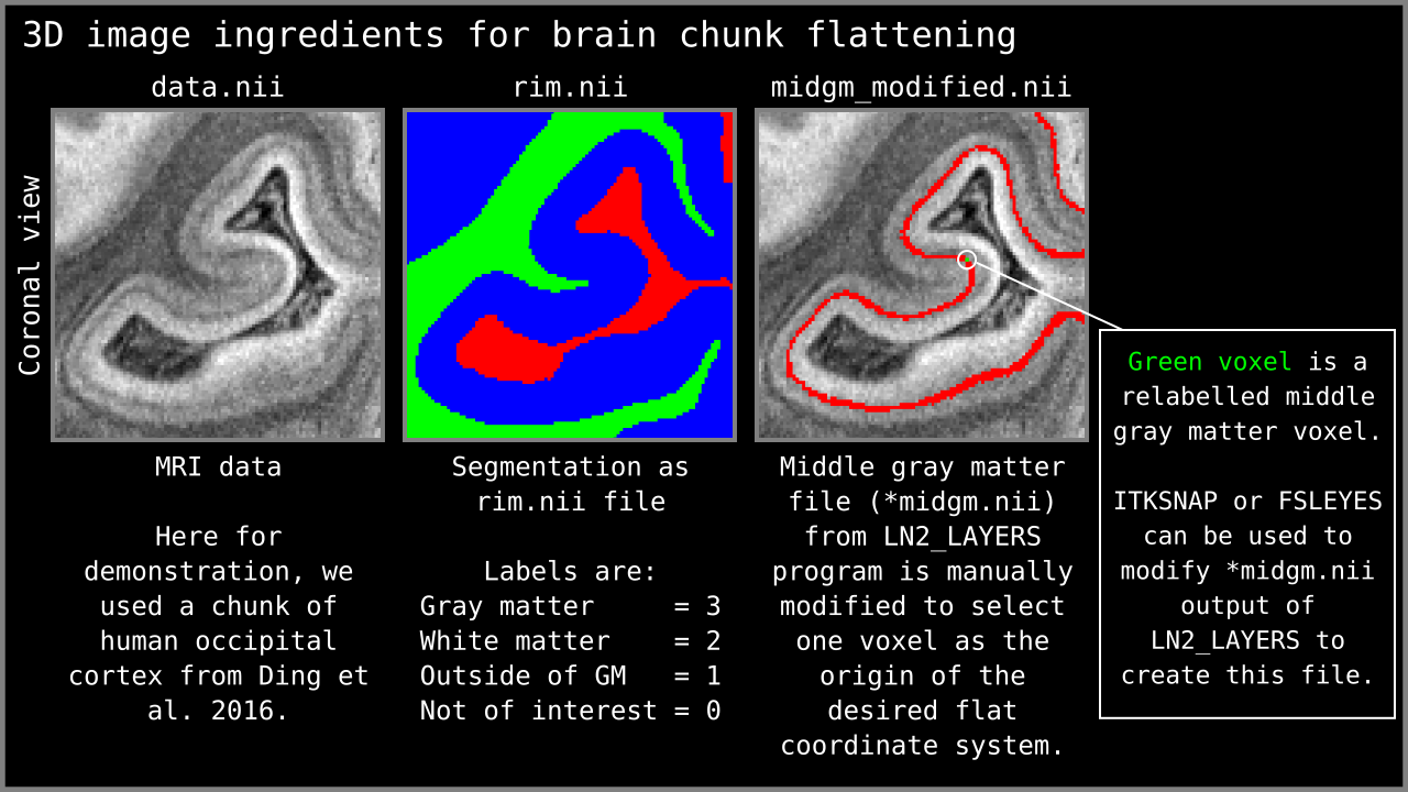
Figure 2: 3D nifti image ingredients for LN2_MULTILATERATE visualized.
Figure 3: MRI data and middle gray matter voxel visualized in 3D. We used MRI data from Ding et al. (2016) and the middle gray matter voxels computed by LN2_LAYERS based on segmentation (rim file shown in Figure 1). We use 3D volume renders to communicate that our ingredients are 3D partial coverage brain images. In other words, we operate on brain chunks.
Rules of the kitchen
- Flattening has to be done in voxel space. We are not allowed to change the input data structure (i.e., no triangular or quad surface meshes). This rule is employed because each time the data structure is changed or augmented, we risk changing certain topographical qualities of our input image (this might be a topic for a future blog post).
Flattening has to accommodate partial coverage. Partial coverage image means that only a partial chunk of the brain is imaged or available as a 3D image.
LN2_MULTILATERATE
From this point onwards we are going to describe the algorithmic steps implemented in the LN2_MULTILATERATE program which is designed to generate flat coordinates.
Step 1: Distances from the origin
Aim: Find the distance of each gray matter voxel relative to the “control point 0” a.k.a. origin voxel.
This step is the first step of parametrizing our middle gray matter voxel (see Figure 3).
Figure 4: The left panel shows where the control point 0 (a.k.a. origin) voxel is located on the middle gray matter voxels. The right panel shows how the geodesic distances are computed with the flooding method.
Step 2: A geodesic disk
Aim: Compute a geodesic disk that contains the middle gray matter voxels that envelop our region of interest.
This computation is done via simple thresholding on the control point 0 distances as computed in the previous step (see Figure 4). For instance, we can determine the size of this disk by changing the `-radius` input of LN2_MULTILATERATE.
Figure 5: The left panel shows the masked geodesis disk around control point 0 relative to the rest of the middle gray matter voxels. The right panel shows how this disk is convoluted in 3D space.
It is important to note that the disk edges should not touch the image edges. In order to check this, we use ITKSNAP to visualize the “*perimeter” output of LN2_MULTILATERATE (see Figure 5).
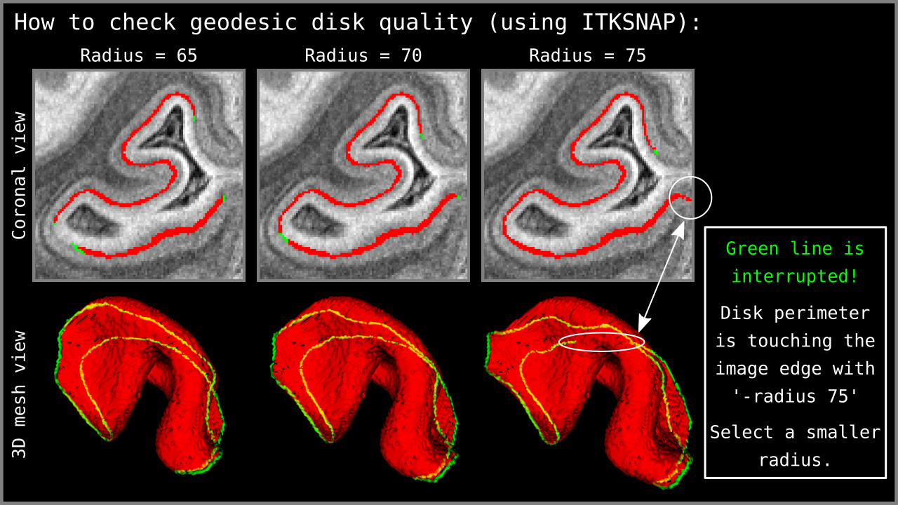
Figure 6: Quality control of the `-radius` parameter using the `*perimeter.nii` output of LN2_MULTILATERATE. Using ITKSNAP, we first load the MRI data as the `main image`; then we load our `*perimeter.nii` file as the `segmentation image` and press the `update` button in the mesh view panel. Looking at the mesh as generated in ITKSNAP, we see a green line that indicates the periphery of our geodesic disk. In the third column above, notice that the disk perimeter generated by the `-radius 75` parameter is discontinuous – the green line is interrupted. If you encounter this behavior, it means that the disk radius is too large for the algorithm to perform correctly. Reduce your radius parameter or – when possible – enlarge your segmented brain chunk region so that the disk can fit into the middle gray matter voxels domain.
Step 4: Four points on the perimeter
Aim: Find four points that are equidistant to each other on the geodesic disk perimeter.
We first find four points on the perimeter of our middle gray matter geodesic disk that we have computed in the previous step. We accomplish this by using our “iterative farthest points” algorithm that was developed for the LN2_COLUMNS program. This time, we specifically operate on the disk perimeter voxels and we only iterate four times to find four points. These four points lie on our disk perimeter and they are equidistant to each other. We call these four points as control points 1, 2, 3, and 4 (remember that we also had a control point 0, which was used in step 1). We compute the middle gray matter geodesic distances from each one of our four control points (visualized in Figure 7).
Figure 7: The left panel shows the geodesic disk (from Figure 4) with control points 1 to 4 as a reference. The right panel shows 4 types of distances (stages indicated in the panel title). These steps are the geodesic distances relative to the control points 1 to 4.
Note that it is possible to determine the control points 1, 2, 3, and 4 manually as visualized in Figure 8. To do this you need to further modify your middle gray matter file. Remember that we have used ITKSNAP to manually determine our control point 0 (see the Ingredients section above). In order the determine the rest of the control points, all you need to do is to select four different middle gray matter voxels and re-label them from “1” to “3” for control point 1; “1” to “4” for control point 2; “1” to “5” for control point 3; and “1” to “6” for control point 4. LN2_MULTILATERATE will automatically recognize this input and will skip the automatic determination of the control points.
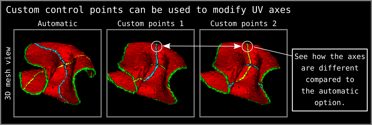
Figure 8: Custom control points can be given to determine the axes of UV coordinates. How to give custom control points as input is explained within the `LN2_MULTILATERATE -help` menu. Note that the 3D mesh view in this figure is coming from ITKSNAP mesh viewing panel after loading the `*_UV_axes.nii.gz` output of LN2_MULTILATERATE as `segmentation file`.
Step 5: The rolling pin maneuver
Aim: Compute two orthogonal axes (lines) geodesically embedded within the middle gray matter voxels.
Subtracting the distances between control point 1 and 2 yields a “zero crossing” line embedded within the middle gray matter voxels. We call this line our first rolling pin axis. Subtracting the distances between control point 3 and 4 yields another “zero crossing” line that is orthogonal to the first one. We call this line our second rolling pin axis. Then, we compute the geodesic distances relative to each one of our rolling pin axes. (visualized in Figure 9).
Figure 9: The left panel shows the geodesic disk (from Figure 4) with pin axes 1 and 2 as a reference. The right panel shows an animation of the geodesic distances being computed relative to the axes depicted in the left panel. The control point 1 and 2 distances are used to determine pin axis 1; and the control point 3 and 4 distances are used to determine pin axis 2.
Step 6: Lateration
Aim: Find the sides of the pin axes.
The pin axis distances that we have computed in the previous step are almost what we want as the final output; however, they lack a crucial detail. We do not yet know which side of the first axis is left or right, and which side of the rolling second axis is up or down. Luckily, this information can be inherited from the previous step, where we have actually computed the signs (plus or minus) of each axis. All we need to do is to swap the sign bit of our pin axis distances. We refer to this step as “lateration”, in reference to the Latin “lateralis” meaning “belonging to the side”. Once this operation has been completed, we have effectively converted our signless rolling pin distances into a coordinate system (see Figure 10).
Figure 10: Flat coordinates (UV coordinates) computed as the result of the lateration step.
Step 7: Cover the cortex thickness
Aim: Propagate the flat coordinates present on the middle gray matter voxel towards the rest of the cortical thickness.
Figure 11: The two panels show the propagation of the flat coordinates (UV coordinates) computed on middle gray matter voxels to the rest of the cortical thickness. The program LN2_MULTILATERATE writes out these UV coordinates as a nifti file (with “*UV_coordinates.nii” suffix).
Final flattening act
At this point we have computed two new coordinates for each voxel. We call these two new coordinates “flat coordinates” or “UV” coordinates. The letters “U” and “V” are inspired by the computer graphics terminology “UV mapping” that refers to finding the flat coordinates of triangular surface meshes (Botsch et al. 2010; Ch. 1.3.3). We also need a third coordinate to encode the cortical depth of each voxel. For this purpose we use the normalized cortical depth measurements computed by using LN2_LAYERS (see the previous post here) with our segmented rim file. We denote this “cortical depth” coordinate with the letter “D”. Now all we need to do is transform each of the voxels’ X, Y, and Z coordinates to the new U, V, and D “flat” coordinates.
To perform the actual flattening, we developed a separate program `LN2_PATCH_FLATTEN`. This little program is implemented separately from LN2_MULTILATERATE because we conceived that there might be other ways to compute the flat coordinates. We decided that it would be advantageous for the LayNii users to be able to freely choose whichever flat coordinate generator they want to employ.
Without further ado, we can visualize the resulting flattening coming from the LN2_MULTILATERATE with various different inputs used with LN2_PATCH_FLATTEN (Figure 12). The ultimate output of LN2_PATCH_FLATTEN is a 3D nifti file that contains the flat brain chunk.
Figure 12: The right panel shows the animated flattening from the convoluted brain chunk to a flat brain chunk. The flat coordinates (U and V coordinates) are computed with `LN2_MULTILATERATE -rim Ding2016_occip_rim.nii.gz -control_points Ding2016_occip_rim_control_point0.nii.gz -radius 70` and the depth coordinates (D coordinate) are computed with `LN2_LAYERS -rim Ding2016_occip_rim.nii.gz -equivol` (the example data can be found in LayNii test_data folder). The right panel shows the resulting flat 3D nifti file generated by the LN2_PATCH_FLATTEN program by using `LN2_PATCH_FLATTEN -coord_uv Ding2016_occip_rim_UV_coordinates.nii.gz -coord_d Ding2016_occip_rim_metric_equivol.nii.gz -bins_u 100 -bins_v 100 -bins_d 21 -values Ding2016_occip_rim_metric_equivol.nii.gz -domain Ding2016_occip_rim_perimeter_chunk.nii.gz` command (files used in this example command is generated by the previous commands LN2_LAYERS and LN2_MULTILATERATE). Note that I have used multiple flat images (MRI intensities, columns, layers) generated by LN2_PATCH_FLATTEN together with the convoluted one in a separate animation script using Nibabel, Numpy and PyVista libraries to communicate what the flattening algorithm is doing.
Algorithm Overview
Understanding an algorithm/recipe gradually develops at different levels of detail. Similar to seeing an island on the horizon and slowly recognizing more and more details as you sail closer, the transition from being a user to a developer requires recognizing the tiniest of details (upon lots of rowing). In this section, we offer *a bird’s eye view* of our algorithm that conveys an intermediate level of detail in between our source code and the rest of this blog post.
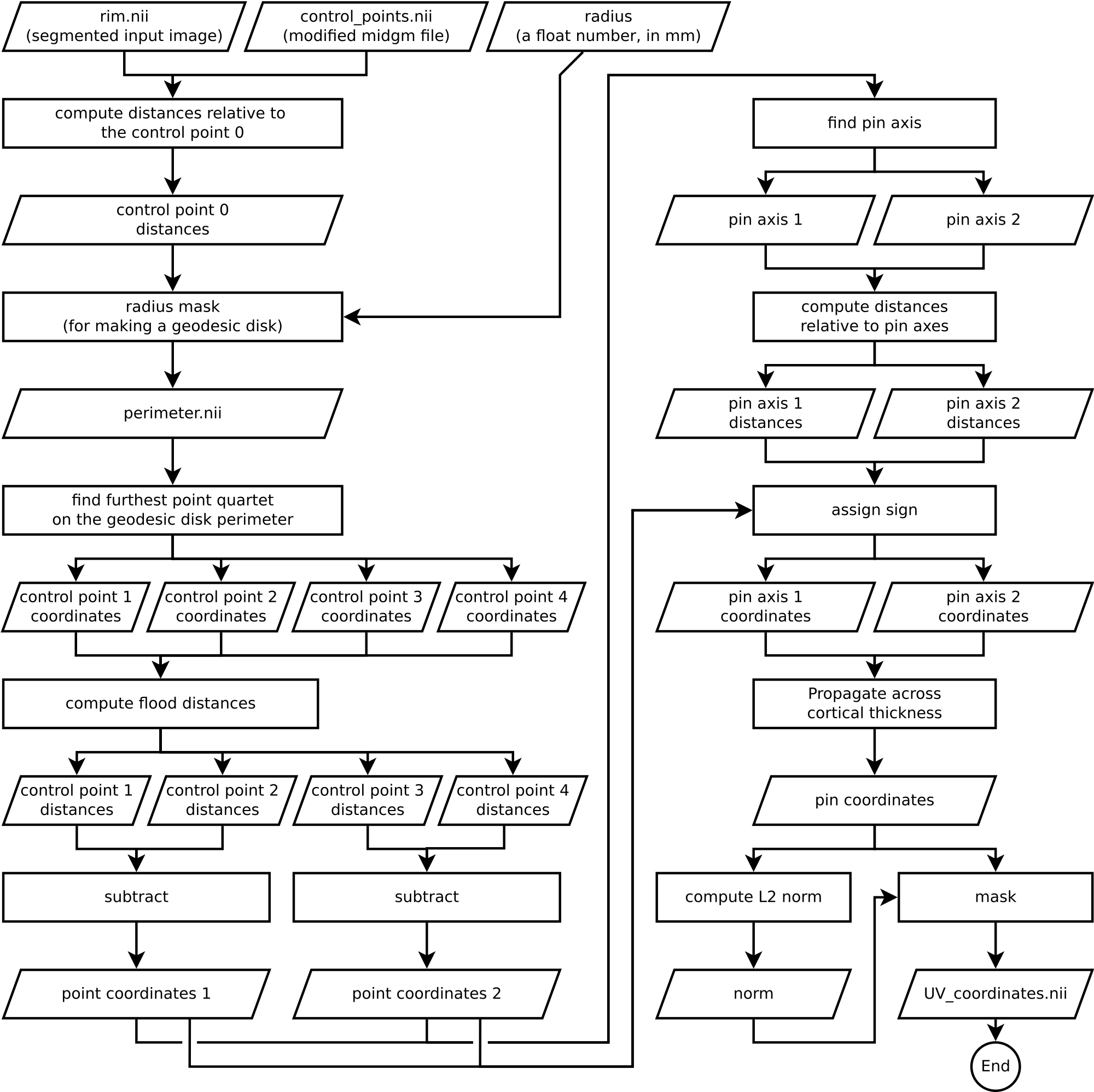
Figure 13. Flowchart of LN2_MULTILATERATE as implemented in LayNii v2.1.0.
How to contribute?
If you have any issues when using LayNii, or want to request a new feature, we are happy to see them posted on our github issues page. Please employ this as your preferred method (instead of sending individual emails to the authors), since fellow researchers might have similar issues and suggestions.
References & Inspirations
- Botsch, M., Kobbelt, L., Pauly, M., Alliez, P., & Levy, B. (2010). Polygon Mesh Processing. In Polygon Mesh Processing. <https://doi.org/10.1201/b10688>
- Ding, S. L., Royall, J. J., Sunkin, S. M., Ng, L., Facer, B. A. C., Lesnar, P., … Lein, E. S. (2016). Comprehensive cellular-resolution atlas of the adult human brain. Journal of Comparative Neurology. [Link]
- Huber, L. (2018). Quick example of cortical unfolding in LayNii. layerfmri.com [Link]
- Yushkevich, P. A., Piven, J., Hazlett, H. C., Smith, R. G., Ho, S., Gee, J. C., & Gerig, G. (2006). User-guided 3D active contour segmentation of anatomical structures: significantly improved efficiency and reliability. NeuroImage, 31(3), 1116–1128. [Link]
Thanks
We thank Rainer Goebel for his encouragement on this endeavor and discussions on various flattening algorithms. We thank Konrad Wagstyl for commenting on the histological data processing perspective. We thank Kendrick Kay for the useful comments and discussion on the general flow and goal of this text.
Visuals
Animations that are not referenced above have been created by the authors and licensed under CC BY 4.0.